Derivation of the AC Power formulae without using phasors, vectors, or complex numbers

I shall prove the AC power formulae without using complex numbers, vectors, or phasors.  Put another way, this proof will support the concept of the power triangle rather than using the power triangle to support the proof.

The plot below shows AC voltage, current, and power when φ = 0 or the voltage and current are in phase:

Note that the power is sinusoidal and has a frequency of twice that of either the voltage or current.  Note further that the power is strictly nonnegative.  The power reaches a peak 2f times per period and reaches a minimum (zero) 2f times per period where f is the frequency of the voltage and/or current.  Since power is the product of current and voltage, these zero values occur when the voltage and current reach zero, and since the voltage and current are in phase, they reach zero at the same time.  In addition, the voltage and current become negative and become positive simultaneously.  In short, the voltage and current are always the same sign when not zero.  Thus their product can never be negative.  This corresponds to a scenario in which there is a purely resistive load.  In such a case, since the power is never negative, energy flows in only one direction.

Below is a plot illustrating the common case of a load with a reactive component.  Specifically, loads with a certain amount of inductive reactance will result in a current which lags the voltage by an angle φ.

Note that within each period of duration 1/f seconds, there are two intervals during which the power is negative.  This is because during these intervals, voltage and current are of different signs.  During one of these intervals, voltage is positive and current is negative.  During the other, voltage is negative and current is positive.  However, for the majority of the time the voltage and current are the same sign, and hence most of the power is positive.  The analytical implications of this positive and negative power will be the central focus of the analysis to follow.

The instantaneous values of voltage and current expressed as time-varying functions are shown below.  These functions are the starting point of our derivations of formulae for real, apparent, and reactive power as well as the power factor.

or

where V is the peak voltage, I is the peak current, 𝜔 is the frequency in radians per second, t is the time in seconds, and φ is the phase difference in radians between the voltage and current.  Then

or

This instantaneous power will be sinusoidal with a frequency of 2𝜔.  The average power will be a value exactly between the maximum and minimum values of this sinusoid, that is to say it will be the numerical average of the maximum and minimum values.  We can find the maximum and minimum values by determining values of P_{INSTANTANEOUS} for which the value of its first derivative is zero.  Furthermore, the maximum and minimum can be distinguished from each other by the sign of the second derivative.

We begin by taking the derivative of the instantaneous power.

Using the product rule:

Using the chain rule:

We use the trigonometric identity:

It will be helpful to rearrange the identity like so:

So

We now seek t = t₁ such that p’(t₁) = 0 because p(t₁) will be an extremum of p(t).  From above, it follows that p’(t) = 0 when 2ωt = φ.  Hence,

Therefore  is either a maximum or minimum value of p(t).  Earlier, I noted that maxima and minima could be distinguished by the numeric sign of the second derivative of the instantaneous power, p’’(t), evaluated at one or more of the extrema.  As it happens, this proves unnecessary at this time.  The value t₁ is a time at which the instantaneous power reaches either a maximum or minimum.  Recall that the instantaneous power curve is a sinusoid with frequency 2ω, or twice the frequency of the voltage and/or current.  Hence if T is the period of the voltage and/or current, then the period of the power is T/2.  Since every sinusoid has two extrema per period, it follows that if the power curve has an extremum at t = t₁, then its next extremum corresponds to t = t₂ = t₁ + T/4.  So we need an expression for T, and we will need it again in later calculations.

The angular frequency ω is defined as ω = 2πf where f is the frequency of the voltage or current in hertz (Hz).  One Hz is defined as one cycle per second.  The hertz is often expressed as 1/sec or 1/s or s^-1.  Therefore ω is expressed in units of inverse-seconds.  We seek the period T expressed in seconds.  Since f is the number of cycles per second, the length of 1 cycle is 1/f.  In other words, T = 1/f.  From the expression for ω at the top of this paragraph, we can solve for f as follows:

so

then

We now have expressions for t₁ and t₂.  We will be evaluating p(t₁) and p(t₂) momentarily.  Analytically, we have not yet identified which of the aforementioned values is a maximum and which is a minimum.  However, we need only add the two values and divide by two to obtain the average power.  Evaluating p(t₁),

Using the trigonometric identity:

Now for p(t₂):

Using the trigonometric identity:

Restating our equation for the average (or real) power,

We have now developed an equation for real power which is valid for any phase angle φ.  Next, we turn our attention to a derivation of the formula for the apparent power.  To do this, we resume our earlier line of inquiry by evaluating the second derivative of the instantaneous power.

By the chain rule:

Earlier, we found the values

and

such that p’(t₁) and p’(t₂) were extrema of the instantaneous power.  Also, we noted that the numeric sign of p’’(t₁) and p’’(t₂) would allow us to determine which extremum was a maximum and which was a minimum.  Proceeding with this:

A positive concavity at t₁ indicates that p(t₁) is a minimum, and a negative concavity at t₂ indicates that p(t₂) is a maximum.  Thus p(t₂) – p(t₁) gives us the range of the instantaneous power, and one-half this value is equal to the amplitude of the instantaneous power, which is synonymous with apparent power.

Please note that the above expression involves φ.  In the next step, φ disappears.  Hence, apparent power is independent of φ.  Nevertheless, the fact that φ was involved in the derivation reinforces the independence of apparent power from φ.

The graphs below illustrate the apparent power for two different values of φ, where
0° < φ < 90°.  The important point to take away is that the amplitude of the power (apparent power) is constant for different values of φ, while the average power (real power) changes and is therefore dependent on φ.

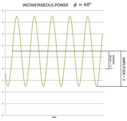
In the graph above for φ = 60°, the average value is 1.5, and the amplitude is 3.  In a practical situation we would say that the real power P = 1.5 watts, and the apparent power S = 3 VA.

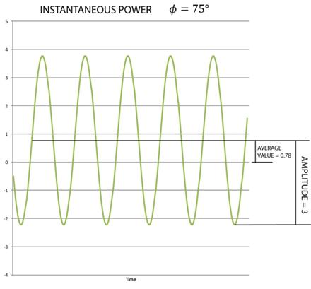
In the second graph above, the average value is 0.78, and the amplitude is still 3.  In a practical situation, we would say that the average power P = 0.78 W, and the apparent power S = 3 VA.  So the apparent power is independent of the phase angle φ, while the real power is dependent on φ.

If we were to look at the extreme cases where φ = 0° and φ = 90°, we would find that the apparent power is still 3 VA in both cases.  The real power, on the other hand, would be 0 W for the case of
φ = 90°.  For the case of φ = 0°, the real power would be 3 W.  Thus for φ = 0°, the real and apparent power have the same magnitude.

The approach we will use to derive the reactive power formula is somewhat different from those we used with apparent and real power.  Not surprisingly, we begin by writing the instantaneous power function.

Our objective will be to manipulate p(t) into the sum of the real and reactive components of instantaneous power.  We now apply the same trigonometric identity we have used previously.

Now here we have two terms, but they are not both functions of time.  We need to press on, but we cannot do this without another trig identity:

We now have two terms which are both functions of t.  By inspection, we can verify that
 is nonnegative, and  has an average value of zero.  This suggests that

and

If we accept that

then by the fact that

it follows that

Note that it does not necessarily follow that p(t) and p_real(t) are equal, but we can be assured that

At this point, a precaution is in order.  One may be tempted to assume that since real power is the average value of p_real(t), then reactive power must be the average value of p_reactive(t).  This is not the case.  As stated above, the average value of p_reactive(t) is zero.  However reactive power is not necessarily zero for all values of φ.  This apparent contradiction may be explained by the fact that the average value of p_real(t) is equal to the amplitude of p_real(t) for all values of φ.  Conversely, the average value of p_reac(t) is not equal to the amplitude of p_reac(t) unless φ = 0°, in which case they are both zero.  Conceptually, the equivalency of the manners by which real and reactive power are defined lies in their respective relationships to the amplitudes of their instantaneous manifestations and not their respective average values.  Thus, in order to derive a formula for reactive power, we must determine the peak value of the instantaneous reactive power.  This peak value will necessarily be equal to the amplitude.

To find the roots which will lead us to the maximum and minimum values of p_reactive(t), we seek t₁ and t₂ such that

and

Where n is an integer.  So

 and

To determine which of these values will lead us to the maximum value of p_reactive(t), we need the second derivative

From above p_reactive(t₂) will be the maximum value.

We have now found the maximum value of the instantaneous reactive power.  And since the average reactive power is zero, the maximum value is also the amplitude of the reactive power.  Therefore,

Along with the reactive power above, we now restate the formulae we derived for real and apparent power so that all three are gathered together in the same place.

By basic trigonometry, given a right triangle having one angle measuring φ, then the length of the hypotenuse, the length of the side opposite the angle φ, and the length of the side adjacent to the angle φ are related according to the following:

and

Observe that

and

These relationships enable us to depict the real, reactive, and apparent power on a right triangle as follows:

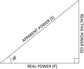
The real, reactive, and apparent power are customarily designated by the following variables:

Another relationship which can be inferred from such a triangle is a result of the Pythagorean Theorem:

or

and

One useful power concept, power factor, remains for us to address.  Its derivation was an incidental byproduct of the above justification of the power triangle.

Thus the power factor is the ratio of real power to apparent power or alternately the cosine of the phase angle.

There can be confusion related to the correct value to use for the phase angle φ when performing power calculations.  To define φ in terms of φ_V and φ_I, we express the instantaneous power in the following way:

The trigonometric identity

allows us to write

Note that the first term above is a constant, and the second term is sinusoidal and has an average value of zero.  As such, the first term is the average value of p(t).  The average value of p(t) is the real power, so

Implies that

In conclusion, be advised that there is a compelling derivation of real power using integration to calculate the average value of the instantaneous power.  Also, phasor representations of voltage, current, and impedance (resistance and reactance respectively) can be used to derive the power formulae.  The stated objective of this document, however, was to do so without using phasors.